This week's set of tasks use a mapping diagram to represent liner functions. This model may not be familiar to some teachers and students but this can be advantage - it allows us to take a fresh look at the characteristics of linear functions and (though we don't do it here) can help us look at the Cartesian graph of linear functions with fresh eyes.
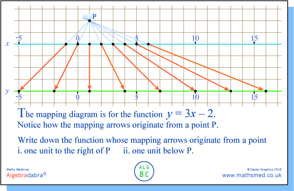
MONDAY: Here we are asked to read a mapping diagram and to determine the function that the given information represents.
TUESDAY: Here we take a more detailed look at Monday's mapping diagram (which was for the function
y = 3
x – 2) and consider how its features can be used to identify the linear function.
WEDNESDAY: I was amazed by this phenomenon when I first came across it (thanks to JH). Of course, as with many mathematical phenomena, the more you think about it the more obvious it becomes. But this one also becomes richer. All in all, an exciting and lovely result!
We can visualise parts i and ii by translating point P
and the arrows one unit to the right (part i) or one unit down (part ii). Alternatively, move both axes one unit to the left (part i) or one unit up (part ii). Which approach do you prefer?
PS: You will probably have noticed that P can be thought of as the
centre of enlargement for the linear function. Image points (ie points on the
y axis) are 3 times the distance from P as object points (ie the corresponding points on the
x axis). So the scale factor of the 'enlargement' is ×3. Similarly, the distance between a pair of points on the
y axis is 3 times the distance of corresponding points on the
x axis.
In part i, the same distance-relationships hold, ie the scale factor is still ×3. However, in part ii the distance-relationships change, and therefore so does the scale factor. Has it got smaller or larger?
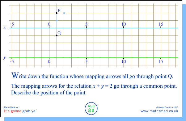
THURSDAY 1: Here we extend the notion that the arrows on mapping diagrams of linear functions emanate from a 'centre of enlargement', by considering centres that lie between the two axes. What does that tell us about the 'scale factor', ie the value of
m in
y = mx + c ?
-
THURSDAY 2 (instead of Good Friday): Here we consider the inverse of our original function.
The inverse takes us back to where we started. One way of representing this there-and-back journey is by adding a second mapping diagram that is a reflection of the original, as here:
Note: the inverse function itself is represented by just the second mapping diagram, but with the axes re-labeled (
x axis at the top,
y axis below), and with the arrows pointing downwards. As can be seen, the 'common point' (or 'centre of enlargement') is vertically below P, two units below the
y axis. The scale factor here is 1/3, and if we look carefully, we can see that 0 is mapped onto 2/3, so the inverse function is
y = 1/3
x + 2/3, or
y = 1/3 (
x + 2). We can verify this algebraically, by transforming the original function
y = 3
x – 2 into
x = .... (and then transposing
x and
y).